Here is the direct way to the products
→ AF08 → LHB 4-8
Let's talk about active electronic filters
• What are ACTIVE FILTERS?
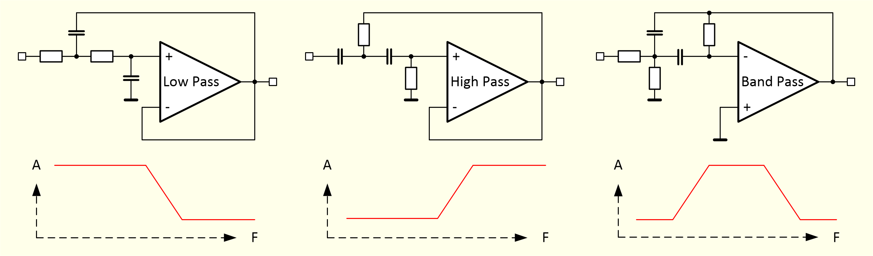
Electronic filters amplify or attenuate certain frequency components in the signal.
In addition to passive filter components (resistors, capacitors), active filters consist of amplifying components (operational amplifiers) to realize the desired frequency response.
• Why do we need LOW PASS FILTERS?
What could happen if you do not limit the bandwidth of your measurement signal before digitization?
First of all a little experiment (analog/digital experts know this, of course):
Take a function generator and a digital oscilloscope, in the example case a simple, older model.
Then we select a sinusoidal signal with 10 kHz for the function generator.
We set the oscilloscope to a horizontal sampling time of 10 µs/div
and the
vertical deflection so that our sinusoidal signal fits well on the display.
You can see one full oscillation of the sine signal (10 kHz = period duration 100 µs).
So far everything is good.
Now we extend the sampling time to 200 µs/div.
The many oscillations can still
be differentiated well.
From a sampling time of 1 ms/div the single oscillations
are no longer
to recognize. With further extension of the sampling time over 50 ms/div
(possibly depending on the oscilloscope model) we suddenly see a
Signal with very low frequency, but full amplitude.
At 500 ms/div (possibly depending on the oscilloscope model) a sine wave can be seen,
almost like at the beginning of the experiment at a sampling time of
20 µs/div.
Which is obviously a signal falsification.
What happened?
Answer: The Nyquist-Shannon sampling theorem (for details please check "wikipedia.com")
has been violated. This means that there was a beat between the frequency of the sine signal (measurement signal)
and the sampling frequency of the oscilloscope.
This generation of an error signal is called aliasing effect.
And the problem is, that this error is not detected during a continuous digitization of measurement signals with
too low sampling rate and cannot be corrected afterwards.
(In newer oscilloscopes there are some possibilities of sample correction for this purpose
which normally cannot be used for longer measuring processes.)
So what can be done to avoid these problems?
The only reasonable way is to limit the bandwidth of the measurement signal.
This ensures that the measurement signal does not conflict with the ADC sampling signal and the
Nyquist-Shannon sampling theorem is not violated.
Active low pass filters are used for this task. The cut-off frequency of the filter
(-3 dB-point), the filter order and the filter characteristics are chosen in such a way that
the amplitude of the measurement signal at the ADC sampling frequency falls below the amplitude corresponding
to the dynamics (number of bits) of the ADC.
Example:
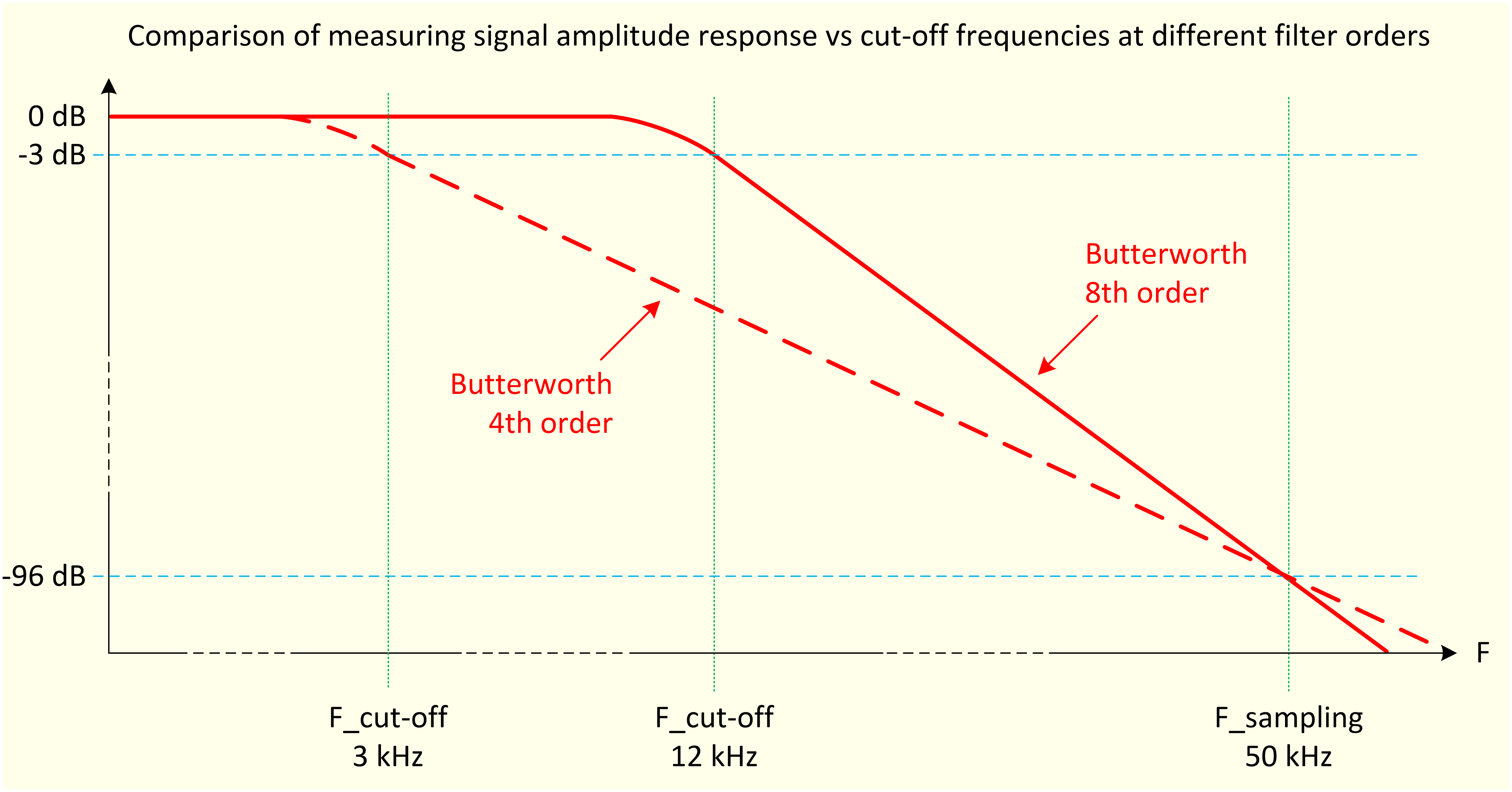
The 16-bit ADC is operated with a sampling rate of 50 kSamles/s. A Butterworth low pass filter of 8th
order is chosen. The -3 dB-point of the lowpass filter must then be at ≤ 12 kHz, so that the amplitude
drop at 50 kHz is below -96 dB
(= 16 * 6 dB/bit dynamic).
With a 4th order Butterorth low pass you would only get a cut-off frequency of approx. 3 kHz.
With a suitable low pass filter, it is therefore ensured that the ADC no longer "sees" any relevant
measurement signal amplitude and therefore cannot generate aliasing products.
And by the way, a beneficial side effect of using low pass filters should not go unmentioned:
The signal noise is reduced.
Over 90% of the active filters we build are of the type:
• Butterworth low pass 8th order, used as anti-aliasing filters.
Conclusion:
Filtering is an essential part of the signal chain of measurement data acquisition.
Insufficient signal filtering can lead to a significant increase in signal noise and to disturbances in the measured values.
• Why are ACTIVE FILTERS expensive?
The filter modules are individually equipped for all values specified by the customer:
• Cut-off frequency (from 50 Hz to 20 kHz)
• Characteristic (Butterworth, Bessel, in special cases also Chebyshev)
• Order (4 or 8 pole).
When designing active filters for measurement technology applications is not
just about the exact observance of the desired cut-off frequency but above all to ensure a smooth
passband without waves and overshoots.
That means a lot of manual work at
• Choosing the right Operational Amplifier (bandwidth, offset)
• Calculation of the values using a filter design program
• Selection (measurement) of the real capacitors
• Recalculation of the resistances based on the actually measured capacitance
values
• Equipping the PCBs with the individually determined components.
And don't forget the test of the finished device.
That is why active filters cannot be easily produced in series, but they are usually always individually
manufactured and therefore relatively EXPENSIVE.
Beside our filter modules → AF08 the following IEPE modules can be equipped with Active Filters (low pass):
• IPE-FM3 IPE-FM3_info.pdf - 386kB [EN]
• IPE-FM6 IPE-FM6_info.pdf - 530kB [EN]
• IPE-DM5 IPE-DM5_info.pdf - 316kB [EN]
• IPE-ISO1 IPE-ISO1_info.pdf - 592kB [EN]
Information -
The IPE-FM3 and IPE-FM6 modules can also be supplied as pure front-mountable active filters: DC-coupled, without IEPE circuitry.
|
Hier ist der direkte Weg zu den Produkten
→ AF08 → LHB 4-8
Lassen Sie uns über aktive elektronische Filter sprechen
• Was sind AKTIVE FILTER?
Elektronische Filter verstärken oder schwächen bestimmte Frequenzanteile im Signal.
Aktive Filter bestehen neben passiven Filterkomponenten (Widerstände, Kondensatoren) aus verstärkenden Komponenten (Operationsverstärkern)
zur Realisierung des gewünschten Frequenzgangs.
• Warum werden TIEFPASS FILTER benötigt?
Was könnte passieren, wenn Sie die Bandbreite Ihres Messsignals vor der Digitalisierung nicht begrenzen?
Vorab ein kleines Experiment (Analog/Digital-Experten kennen das natürlich):
Nehmen wir einen Funktionsgenerator und ein digitales Oszilloskop,
im Beispielfall ein einfaches, älteres Modell.
Dann wählen wir beim Funktionsgenerator ein Sinussignal mit 10kHz.
Wir stellen das Oszilloskop auf eine horizontale Abtastzeit von 10µs/div
und die vertikale Ablenkung so, dass unser Sinussignal gut auf das Display passt.
Zu sehen ist eine volle Schwingung des Sinussignals (10kHz = Periodendauer 100µs).
Soweit ist alles gut.
Jetzt verlängern wir die Abtastzeit auf 200µs/div.
Die vielen Schwingungen sind noch gut zu differenzieren.
Ab einer Abtastzeit von 1ms/div sind die einzelnen Schwingungen nicht mehr
zu erkennen. Bei weiterer Verlängerung der Abtastzeit über 50ms/div
(event. abhängig vom Oszilloskop-Modell) hinaus sehen wir plötzlich ein
Signal mit sehr niedriger Frequenz, aber voller Amplitude.
Bei 500ms/div (event. abhängig vom Oszilloskop-Modell) ist eine
Sinus-
schwingung zu sehen, fast wie zu Beginn des Experiments bei einer Abtastzeit von 20µs/div.
Was offensichtlich eine Signalverfälschung darstellt.
Was ist geschehen?
Antwort: Das Nyquist-Shannon-Abtasttheorem (für Details bitte bei "wikipedia.de" nachsehen) wurde verletzt.
Das bedeutet, dass eine Schwebung entstand zwischen der Frequenz des Sinussignals (Messsignals)
und der Abtastfrequenz des Oszilloskops.
Diese Bildung eines Fehlersignals wird Aliasing-Effekt genannt.
Und das Problem ist, dass diese Fehler bei einer kontinuierlichen Digitalisierung von Messsignalen mit einer
zu geringen Abtastrate nicht erkannt und nicht nach-träglich behoben werden kann.
(In neueren Oszilloskopen stehen dafür einige Möglichkeiten der Abtastkorrektur zur
Verfügung, die aber normalerweise bei längeren Messvorgängen nicht angewandt werden können.)
Was ist also zu tun um diese Probleme zu umgehen?
Der einzig sinnvolle Weg ist, das Messsignal in der Bandbreite zu begrenzen.
Damit läst sich erreichen, dass das Messsignal nicht mit dem ADC-Abtastsignal in Konflikt gerät und das
Nyquist-Shannon-Abtasttheorem nicht verletzt wird.
Für diese Aufgabe werden aktive Tiefpass-Filter eingesetzt. Wobei die Grenz-
frequenz des Filters
(-3dB-Punkt), die Filter-Ordnung und Filter-Charakteristik so gewählt wird, dass die Amplitude
des Messsignal bei der Abtastfrequenz (ADC-Abtastrate) unter die Amplitude fällt, die der Dynamik (Anzahl der Bits) des ADCs entspricht.
Beispiel:
Der 16-Bit ADC wird mit einer Abtastrate von 50kSamles/s betrieben. Gewählt wird ein Butterworth-Tiefpass
8. Ordnung. Der -3dB-Punkt des Tiefpass-Filters muss dann bei ≤ 12kHz liegen, damit der Amplitudenabfall
bei 50kHz unter -96dB (= 16 * 6dB/Bit Dynamik) liegt.
Bei einem Butterworth-Tiefpass 4. Ordnung käme man hier nur auf eine Grenzfrequenz von ca. 3kHz.
Mit einem passenden Tiefpass-Filter wird also gewährleistert, dass der ADC keine relevante Messsignal-Amplitude
mehr "sieht" und deshalb keine Aliasing-Produkte generieren kann.
Und nebenbei soll ein vorteilhafter Nebeneffekt beim Einsatz von Tiefpass-Filtern nicht unerwähnt bleiben:
Das Signalrauschen wird reduziert.
Über 90% der von uns gebauten Aktiven Filter sind vom Typ:
• Butterworth Tiefpass 8. Ordnung, als Anti-Aliasing-Filter verwendet.
Fazit:
Filtern ist ein wesentlicher Bestandteil der Signalkette der Messdatenerfassung.
Unzureichende Signalfilterung kann zu einem erheblichen Anstieg des Signal- rauschens und zu Störungen in den Messwerten führen.
• Warum sind AKTIVE FILTER teuer?
Die Filtermodule werden individuell für alle vom Kunden spezifizierten Werte bestückt:
• Grenzfrequenz (von 50Hz bis 20kHz)
• Charakteristic (Butterworth, Bessel, in besonderen Fällen auch Chebyshev)
• Ordnung (4 oder 8 Pole).
Bei der Konzeption von Aktiven Filtern ist für Messtechnikanwendungen nicht nur auf
die exakte Einhaltung der gewünschten Grenzfrequenz sondern vor allem auf einen
glatten Durchlassbereich ohne Wellen und Überschwinger zu achten.
Das bedeutet jeweils viel Handarbeit bei der
• Wahl des passenden Operationsverstärkers (Bandbreite, Offset)
• Berechnung der Werte mittels Filter-Design-Programm
• Selektion (Ausmessen) der realen Kondensatoren
• Neuberechnung der Widerstände anhand der tatsächlich gemessenen
Kapazitätswerte
• Bestückung der Leiterplatten mit den individuell ermittelten Komponenten.
Und nicht zu vergessen der Test des fertigen Gerätes.
Deshalb sind Aktive Filter nicht gut in Serie herstellbar, sondern sind praktisch immer
individuell gefertigt und damit relativ TEUER.
Neben unseren Filter-Modulen → AF08 sind folgende IEPE-Module mit Aktiven Filtern (Tiefpass) ausrüstbar:
• IPE-FM3 IPE-FM3_info.pdf - 386kB [EN]
• IPE-FM6 IPE-FM6_info.pdf - 530kB [EN]
• IPE-DM5 IPE-DM5_info.pdf - 316kB [EN]
• IPE-ISO1 IPE-ISO1_info.pdf - 592kB [EN]
Information -
Die Module IPE-FM3 und IPE-FM6 können auch als reine frontmontierbare
Aktive Filter geliefert werden: DC-gekoppelt, ohne IEPE- Schaltungsteil.
|